Tiny-TPU: the why and how

A TPU is an application specific chip (ASIC) designed by Google to make inferencing (using) and training ML models faster and more efficient. Whereas a GPU can be used to render frames AND run ML workloads, a TPU can only perform math operations, allowing it to be better at what it's designed for. Naturally, trying to master a single task is much easier and will yield better results than trying to master multiple tasks and the TPU strongly employs this philosophy.

Quick primer on hardware design:

In hardware, the unit of time we're dealing with is called a clock cycle. This is an arbitrary period of time that we can set, as developers, to meet our requirements. Generally, a single clock cycle can range from 1 picosecond (ps) to 1 nanosecond (ns) and any operations we run will be executed BETWEEN clock cycles.

The language we use to describe hardware is called Verilog. It's a hardware description language that allows us to describe the behaviour of a given hardware module (similar to functions in software), but instead of executing as a program, it synthesizes into boolean logic gates (AND, OR, NOT, etc.) that can be combined to build the digital logic for any chip we want. Here's a simple example of an addition in Verilog:

module add (
    input wire clk,
    // reset signal to reset the module
    input wire rst,

    // registers to hold the input and output values
    input reg a,
    input reg b,
    output reg c
  );
    
    always @(posedge clk) begin 

    // everything in this block will be executed every clock cycle
    
      if (rst) begin
      // reset the output to 0 when the reset signal is high
        c <= 0; 
      end else begin
        // add the two inputs and store the result in the output
        c <= a + b; 
      end
    end

endmodule

In the example above, the value of the signal b at the next clock cycle is set to the current value of the signal a. You'll find that in most cases, signals (variables) are updated in sequential clock cycles, as opposed to immediate updates like you would find in software design.

Specifically, the TPU is very efficient at performing matrix multiplications, which make up 80-90% of the compute operations in transformers (up to 95% in very large models) and 70-80% in CNNs. Each matrix multiplication represents the calculation for a single layer in an MLP, and in deep learning, we have many of these layers, making TPUs increasingly efficient for larger models.

When we started this project, all we knew was that the equation y = mx + b is the foundational building block for neural networks. However, we needed to fully UNDERSTAND the math behind neural networks to build other modules in our TPU. So before we started writing any code, each of us worked out the math of a simple 2 -> 2 -> 1 multi-layer perceptron (MLP).

Why XOR?

The reason we chose this specific network is because we were targeting inference and training for the XOR problem (the "hello world" of neural networks). The XOR problem is one of the simplest problems a neural network can solve. All other gates (AND, OR, etc) can predict the outputs from its inputs using just one linear line (one neuron) to separate which inputs correspond to a 0 and which ones correspond to a 1. But to classify all XOR, an MLP is needed, since it requires curved decision boundaries, which can't be achieved with ONLY linear equations.

Batching and dimensions

Now, say we want to do continuous inference (i.e. self driving car making multiple predictions a second). That would imply that we're sending multiple pieces of data at once. Since data is inherently multidimensional and has many features, we would have matrices with very large dimensions. However, the XOR problem simplifies the dimensions for us, as there are only two features (0 or 1) and 4 possible pieces of input data (four possible binary combinations of 0 and 1). This gives us a 4x2 matrix, where 4 is the number of rows (batch size) and 2 is the number of columns (feature size).

Another simplification we're making for our systolic array example here is that we'll use a 2x2 instead of the 256x256 array used in the TPUv1. However, the math is still faithful so nothing is actually dumbed down, rather scaled down instead.

The first step in the equation is multiplying m with x, which, in matrix form, would be $\mathbf{X}\mathbf{W}^T$.

How can we perform matrix multiplication in hardware? Well, we can use a unit called the systolic array!

Systolic array and PEs

The heart of a TPU is a unit called the systolic array.^[2] It consists of individual building blocks called Processing Elements (PE) which are connected together in a grid-like structure. Each PE performs a multiply-accumulate operation, meaning it multiplies an incoming input X with a stationary weight W^[3] and adds it to an incoming accumulated sum, all in the same clock cycle.

always_ff @(posedge clk or posedge rst) begin
        if (rst) begin
            input_out <= 0;
            psum_out <= 0;
            weight_reg <= 0;
        end else if (load_weight) begin
            weight_reg <= weight;
        end else if (start) begin
            input_out <= input_in;
            // the main multiply-accumulate operation
            psum_out <= (input_in * weight_reg) + psum_in;
        end
    end

Systolic matrix multiplication

When these PEs are connected together, they can be used to perform matrix multiplication systolically, meaning multiple elements of the output matrix can be calculated every clock cycle. The inputs enter the systolic array from the left and move to the neighbouring PE to the right, every clock cycle. The accumulated sums start with the multiplication output from the first row of PEs, move downwards, and get added to the products of each successive PE, until they up at the last row of PEs where they become an element of the output matrix.

Because of this single unit (and the fact that matrix multiplications dominate the computations performed in models), TPUs can very easily inference and train any model.

Worked example

Now let's walk through the example of our XOR problem:

Our systolic array takes two inputs: the input matrix and the weight matrix. For our XOR network, we initialize with the following weights and biases:

Input and weight scheduling

To input our input batch within the systolic array, we need to:

• Rotate our X matrix by 90 degrees







• STAGGER the inputs (delay each row by 1 clock cycle)^[4]

To input our weight matrix: we need to:

• Stagger the weight matrix (similar to the inputs)



• Transpose it!

Note that the rotating and staggering don't have any mathematical significance — they are simply required to make the systolic array work. The transpoing too is just for mathematical bookkeeping – it's required to make the matrix math work because of how we set up our weight pointers within the neural network drawing.

Staggering and FIFOs

To perform the staggering, we designed near-identical accumulators for the weights and inputs that would sit above and to the left of the systolic array, respectively.

Since the activations are fed into the systolic array one-by-one, we thought a first-in-first-out queue (FIFO) would be the optimal data storage option. There was a slight difference between a traditional FIFO and the accumulators we built, however. Our accumulators had 2 input ports — one for writing weights manually to the FIFO and one for writing the previous layer's outputs from the activation modules BACK into the input FIFOs (the previous layer's outputs are inputs for the current layer).

We also needed to load the weights in a similar fashion for every layer, so we replicated the logic for the weight FIFOs, without the second port.

Systolic array matrix multiplication

clk 0

Bias and activation

The next step in the equation is adding the bias. To do this in hardware, we need to create a bias module under each column of the systolic array. We can see that as the sums move out of the last row within the systolic array, we can immediately stream them into our bias modules to compute our pre-activations. We will denote these values with the variable Z.

Now our equation is starting to look a lot like what we've learned in high school –but just in multidimensional form, where each column that streams out of the systolic array represents its own feature!

Next we have to apply the activation, for which we chose Leaky ReLU.^[5] This is also an element-wise operation, similar to the bias, meaning we need an activation module under every bias module (and by proxy under every column of the systolic array) and we can stream the outputs of our bias modules into the activation modules immediately.We will denote these post-activation values with H.

Systolic array with bias and leaky ReLU

clk 0

Pipelining

Now you might be asking – why don't we merge the bias term and the activation term in one clock cycle? Well, this is because of something called pipelining! Pipelining allows multiple operations to be executed simultaneously across different stages of the TPU —instead of waiting for one complete operation to finish before starting the next, you break the work into stages that can overlap. Think of it like an assembly line: while one worker (activation module) processes a part, the previous worker (bias module) is already working on the next part. This keeps all of the modules busy rather than having them sit idle waiting for the previous stage to complete. It also affects the speed at which we can run our TPU — if we have one module that tries to squeeze many operations in a single cycle, our clock speed will be bottlenecked by that module, as the other modules can only run as fast as that single module. Therefore, it's efficient and best practice to split up operations into individual clock cycles as much as possible.

Another mechanism we used to run our chip as efficiently as possible, was a propagating "start" signal, which we called a travelling chip enable (denoted by the purple dot). Because everything in our design was staggered, we realized that we could very elegantly assert a start signal for a single clock cycle at the first accumulator and have it propagate to neighbouring modules exactly when they needed to be turned on.

This would extend into the systolic array and eventually the bias and activation modules, where neighbouring PEs and modules, moving from the top left to the bottom right, were turned on in consecutive clock cycles. This ensured that every module was only performing computations when it was required to and wasn't wasting power in the background.

Double buffering

Now, we know that starting a new layer means we must compute the same $\mathbf{X}\mathbf{W}^T$ using a new weight matrix. How can we do this if our systolic array is weight-stationary? How can we change the weights?

While thinking about this problem, we came across the idea of double buffering, which originates from video games. The reason why double buffering exists is to prevent something called screen tearing on your monitor. Ultimately, pixels take time to load and we'd like to "hide away" that time somehow. And if you paid attention, this is the exact same problem we're currently facing with the systolic array. Fortunately, video game designers have already come up with a solution for this problem. By adding a second "shadow" buffer, which holds the weights of the next layer while the current layer is being computed on, we can load in new weights during computation, cutting the total clock cycle count in half.

To make this work, we also needed to add some signals to move the data. First, we needed a signal to indicate when to switch the weights in the shadow buffer and the active buffer. We called this signal the "switch" signal (denoted by the blue dot) and it copied the values in the shadow buffer to the active buffer. It propagated from the top left of the systolic array to the bottom right (the same path as the travelling chip enable, but only within the systolic array). We then needed one more signal to indicate when we wanted to move the weights down by one row and we called this the "accept" flag (denoted by the green dot) because each row is ACCEPTING a new set of weights. This would move the new weights into the top row of the systolic array, as well as each row of weights down into the next row of the systolic array. These two control flags worked in tandem to make our double buffering mechanism work.

clk 0

If you haven't already noticed, this allows the systolic array to do something powerful…continuous inference!!! We can continuously stream in new weights and inputs and compute forward pass for as many layers as we want. This touches into a core design philosophy of the systolic array: we want to maximize PE usage. We always want to keep the systolic array fed!

For Layer 2, the outputs from Layer 1 ($\mathbf{H}_1$) now become our inputs:

$$\mathbf{z}_2 = \mathbf{H}_1\mathbf{W}_2^T = \begin{bmatrix} -0.2470 & \phantom{-}0.1890 \\[0.2em] -0.5366 & \phantom{-}0.6124 \\[0.2em] -0.0977 & \phantom{-}0.2803 \\[0.2em] -0.3873 & \phantom{-}0.7037 \end{bmatrix} \begin{bmatrix} \phantom{-}0.5266 \\[0.2em] \phantom{-}0.2958 \end{bmatrix} = \begin{bmatrix} -0.0741 \\[0.2em] -0.1014 \\[0.2em] \phantom{-}0.0315 \\[0.2em] \phantom{-}0.0042 \end{bmatrix}$$

Adding bias and applying activation:

$$\mathbf{z}_2 = \mathbf{z}_2 + \mathbf{b}_2 = \begin{bmatrix} \phantom{-}0.5617 \\[0.2em] \phantom{-}0.5344 \\[0.2em] \phantom{-}0.6673 \\[0.2em] \phantom{-}0.6400 \end{bmatrix}$$

$$\hat{\mathbf{y}} = \mathbf{h}_2 = \text{LeakyReLU}_{0.5}(\mathbf{z}_2) = \begin{bmatrix} \phantom{-}0.5617 \\[0.2em] \phantom{-}0.5344 \\[0.2em] \phantom{-}0.6673 \\[0.2em] \phantom{-}0.6400 \end{bmatrix}$$

All values are positive, so they pass through unchanged. These are our final predictions for the XOR problem!

Forward pass walkthrough (with double buffering)

clk 0

Control unit and ISA

Our final step for inference was making a control unit to use a custom instruction set (ISA) to assert all of our control flags and load data through a data bus. Including the data bus, our ISA was 24 bits long and it made our testbench more elegant as we could pass a single string of bits every clock cycle, rather than individually setting multiple flags.

We then put everything together and got inference completely working! This was a big milestone for us and we were very proud about what we had accomplished.

Backpropagation and training

Ok we've solved inference — but what about training? Well here's the beauty: We can use the same architecture we use for inference for training! Why? Because training is just matrix multiplications with a few extra steps.

Here's where things get really exciting. Let's say we just ran inference on the XOR problem and got a prediction that looks something like [0.8, 0.3, 0.1, 0.9] when we actually wanted [1, 0, 0, 1]. Our model is performing poorly! We need to make it better. This is where training comes in. We're going to use something called a loss function to tell our model exactly how poorly it's doing. For simplicity, we chose Mean Squared Error (MSE) — think of it like measuring the "distance" between what we predicted and what we actually wanted, just like how you might measure how far off target your basketball shot was. Let's denote the loss with L.

$$\mathcal{L} = \frac{1}{N}\sum_{i=1}^{N}(y_i - \hat{y}_i)^2$$

where $y_i$ is the target output, $\hat{y}_i$ is our prediction, and $N$ is the number of samples

For our XOR example, with predictions $\hat{\mathbf{y}} = [0.5617, 0.5344, 0.6673, 0.6400]^T$ and targets $\mathbf{y} = [0, 1, 1, 0]^T$:

$$\mathcal{L} = \frac{1}{4}[(0 - 0.5617)^2 + (1 - 0.5344)^2 + (1 - 0.6673)^2 + (0 - 0.6400)^2]$$

$$\mathcal{L} = \frac{1}{4}[0.3155 + 0.2168 + 0.1107 + 0.4096] = 0.2631$$

This loss value tells us how far off our predictions are from the true XOR outputs.

So right after we finish computing our final layer's activations (let's call them $\mathbf{H}_2$), we immediately stream them into a loss module to calculate just how bad our predictions are. These loss modules sit right below our activation modules, and we only use them when we've reached our final layer. But here's the key insight: you don't actually need to calculate the loss value itself to train. You just need its derivative. Why? Because that derivative tells us which direction to adjust our weights to make the loss smaller. It's like having a compass that points toward "better performance."

The magic of the chain rule

This is where calculus enters the picture. To make our model better, we need to figure out how changing each weight affects our loss. The chain rule lets us break this massive calculation into smaller, manageable pieces.

The chain rule for gradients:

$$\frac{\partial \mathcal{L}}{\partial \mathbf{W}} = \frac{\partial \mathcal{L}}{\partial \mathbf{Z}} \cdot \frac{\partial \mathbf{Z}}{\partial \mathbf{W}}$$

This allows us to compute gradients layer by layer, propagating them backwards through the network

Let's trace through what happens step by step.

1. Calculate $\frac{\partial \mathcal{L}}{\partial \mathbf{H}_2}$ - how much the loss changes with respect to our final activations.


2. Compute $\frac{\partial \mathbf{H}_2}{\partial \mathbf{Z}_2}$ by taking the derivative of the activation (leaky ReLU in our case).


3. Compute $\frac{\partial \mathbf{Z}_2}{\partial \mathbf{W}_2}$, $\frac{\partial \mathbf{Z}_2}{\partial \mathbf{H}_2}$

Since all elements of $\mathbf{z}_2$ are positive, the LeakyReLU gradient is 1:

The beautiful symmetry of forward and backward pass

After drawing out the entire computational graph, we discovered something remarkable: the longest chain in backpropagation closely resembles forward pass! In forward pass, we multiply activation matrices with transposed weight matrices. In backward pass, we multiply gradient matrices with weight matrices (untransposed). It's like looking in a mirror!

Once we have all of these individual derivatives, we can multiply them together to find any derivative with respect of the loss (i.e. $\frac{\partial \mathcal{L}}{\partial \mathbf{H}_2} \cdot \frac{\partial \mathbf{H}_2}{\partial \mathbf{Z}_2} \cdot \frac{\partial \mathbf{Z}_2}{\partial \mathbf{W}_2}$ gives us $\frac{\partial \mathcal{L}}{\partial \mathbf{W}_2}$).

After that, we have to compute the activation derivative $\frac{\partial \mathbf{H}_2}{\partial \mathbf{Z}_2}$, for which the formula is $\frac{\partial \text{LeakyReLU}_{\alpha}(\mathbf{Z}_2)}{\partial \mathbf{Z}_2} = \begin{cases} 1 & \text{if } \mathbf{Z}_2 > 0 \\[0.3em] \alpha & \text{if } \mathbf{Z}_2 \leq 0 \end{cases}$. This is also an element-wise computation, meaning we can structure it exactly like the loss module (and bias and activation modules), but it will perform a different calculation. One important note about this module, however, is that it requires the activations we computed during forward pass.

Now you might be wondering — how do we actually compute derivatives in hardware? Let's look at Leaky ReLU as an example, since it's beautifully simple but demonstrates the key principles. Remember that Leaky ReLU applies different operations based on whether the input is positive or negative. The derivative follows the same pattern: it outputs 1 for positive inputs and a small constant (we used 0.01) for negative inputs.

always @(posedge clk) begin
    if (rst) begin
        output <= 0;
    end else begin
        output <= (input > 0) ? input : 0.01 * input;
    end
end

What's beautiful about this is that it's just a simple comparison – no complex arithmetic needed. The hardware can compute this derivative in a single clock cycle, keeping our pipeline flowing smoothly. This same principle applies to other activation functions: their derivatives often simplify to basic operations that hardware can execute very efficiently. This insight led us to compute the long chain first — getting all our$\frac{\partial \mathcal{L}}{\partial \mathbf{Z}_n}$ gradients just like we computed activations in forward pass. We could cache these gradients and reuse them, following the same efficient pattern we'd already mastered.

You'll notice a really cool pattern emerging: all these modules that sit underneath the systolic array process column vectors that stream out one by one. This gave us the idea to unify them into something we called a vector processing unit (VPU) – because that's exactly what they're doing, processing vectors element-wise!^[6]

Not only is this more elegant to work with, it's also useful when we scale our TPU beyond a 2x2 systolic array, as we'll have N number of these modules (N being the size of the systolic array), each of which we would have to interface with individually. Unifying these modules under a parent module makes our design more scalable and elegant!

Additionally, by incorporating control signals for each module, which we call the VPU pathway bits, we can selectively enable or skip specific operations. This makes the VPU flexible enough to support both inference and training. For instance, during the forward pass, we want to apply biases and activations but skip computing loss or activation derivatives. When transitioning to the backward pass, all modules are engaged, but within the backward chain we only need to compute the activation derivative. Due to pipelining, all values that flow through the VPU pass through each of the four modules, and any unused modules simply act as registers, forwarding their inputs to outputs without performing computation.

The next few derivatives are interesting because we can actually use matrix multiplication (and the systolic array!) to compute the derivatives with the help of these three identities:

1. If we have $\mathbf{Z} = \mathbf{X}\mathbf{W}^T$ and take its derivative with respect to the weights, we get $\frac{\partial \mathbf{Z}}{\partial \mathbf{W}} = \mathbf{X}$
2. If we have $\mathbf{Z} = \mathbf{X}\mathbf{W}^T$ and take its derivative with respect to the inputs $\mathbf{X}$, we get $\frac{\partial \mathbf{Z}}{\partial \mathbf{X}} = \mathbf{W}^T$ (just the weight matrix transposed)
3. For the bias term, the derivative is simply 1.

This means that we can multiply the previous $\frac{\partial \mathbf{H}}{\partial \mathbf{Z}}$ with $\mathbf{X}$, $\mathbf{W}^T$, and 1 to get $\frac{\partial \mathbf{H}}{\partial \mathbf{W}}$, $\frac{\partial \mathbf{H}}{\partial \mathbf{X}}$, and $\frac{\partial \mathbf{H}}{\partial \mathbf{b}}$, respectively, and we can multiply all of these by $\frac{\partial \mathcal{L}}{\partial \mathbf{H}}$ to get the gradients of the loss with respect to all of our second layer parameters. And because all of the gradients are actually gradient matrices, we can use the systolic array!

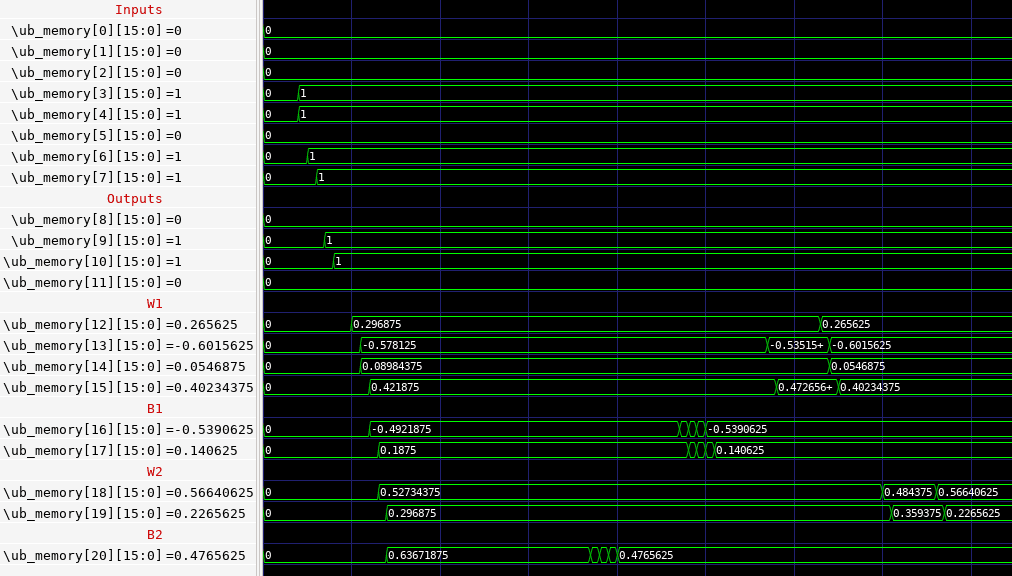
Now something to note about the activation derivative $\frac{\partial \mathbf{H}_2}{\partial \mathbf{Z}_2}$ and the weight derivative $\frac{\partial \mathbf{Z}}{\partial \mathbf{W}}$ is that they both require the post-activations (H) we calculate during forward pass. This means we need to store the outputs of every layer in some form of memory to be able to perform training. Here's where we created a new scratchpad memory module^[7] which we called the unified buffer (UB).^[8] This lets us store our H values immediately after we compute them during forward pass.

We realized that we can also get rid of the input and weight accumulators, as well as manually loading the bias and leak factors into their respective modules, by using the UB to store them. This is also better practice, rather than loading in new data every clock cycle with the instruction set. Since we want to access two values (2 inputs or 2 weights for each row/col of the systolic array) at the same time, we added TWO read and write ports. We did this for each data primitive (inputs, weights, bias, leak factor, post activations) to minimize data contention since we have many different types of data.

To read values, we supply a starting address and the number of values, we supply a starting address and the number of locations we want the UB to read and it will read 2 values every clock cycle. Writing is a similar mechanism, where we specify which values we want to write to each of the two input ports. The beauty in the read mechanism is that it runs in the background once we supply a starting address until the number of locations given are read, meaning we only need to provide an instruction for this every few clock cycles.

At the end of the day, not having these mechanisms wouldn't break the TPU — but they allow us to always keep the systolic array fed, which is a core design principle we couldn't compromise.

While we were working on this, we realized we could make one last small optimization for the activation derivative module — since we only use the $\mathbf{H}_2$ values once (for computing $\frac{\partial \mathbf{H}_2}{\partial \mathbf{Z}_2}$), we created a tiny cache within the VPU instead of storing them in the UB. The rest of the $\mathbf{H}$ values will be stored in the UB because they're needed to compute multiple derivatives.

This is what the new TPU architecture, modified to perform training, looks like:

Now we can do backpropagation!

Going back to the computational graph, we discovered something remarkable: the longest chain in backpropagation closely resembles forward pass! In forward pass, we multiply activation matrices with transposed weight matrices. In backward pass, we multiply gradient matrices with weight matrices (untransposed). It's like looking in a mirror!

This insight led us to compute the long chain of the computational graph first (highlighted in yellow) – getting all our $\frac{\partial \mathcal{L}}{\partial \mathbf{Z}_n}$ gradients just like we computed activations in forward pass. We could cache these gradients and reuse them, following the same efficient pattern we'd already mastered.

We create a loop where we:

1. Fetch a bridge node ( $\frac{\partial \mathcal{L}}{\partial \mathbf{Z}_n}$) from our unified buffer
2. Fetch the corresponding $\mathbf{H}_n$ matrix, also from unified buffer
3. Stream these through our systolic array to compute the weight gradients

Backward pass through second hidden layer

clk 0

And here's where something really magical happens: we can stream these weight gradients directly into a gradient descent module while we're still computing them! This module takes the current weights stored in memory and updates them using the gradients.

No waiting around — everything flows like water through our pipeline.

You might be wondering: "We've used our matrix multiplication identities for the long chain and weight gradients — how do we calculate bias gradients?" Well, we've actually already done most of the work! Since we're processing batches of data, we can simply sum (the technical term is "reduce") the $\frac{\partial \mathcal{L}}{\partial \mathbf{Z}_n}$ gradients across the batch dimension. The beauty is that we can do this reduction right when we're computing the long chain — no extra work required!

With all these new changes and control flags, our instruction is significantly longer — 94 bits in fact! But we can confirm that every single one of these bits is needed and we ensured that we couldn't make the instruction set any smaller without compromising the speed and efficiency of the TPU.

Putting it all together

By continuing this same process iteratively – forward pass, backward pass, weight updates – we can train our network until it performs exactly how we want. The same systolic array that powered our inference now powers our training, with just a few additional modules to handle the gradient computations.

What started as a simple idea about matrix multiplication has grown into a complete training system. Every component works together in harmony: data flows through pipelines, modules operate in parallel, and our systolic array stays fed with useful work.